Introduction

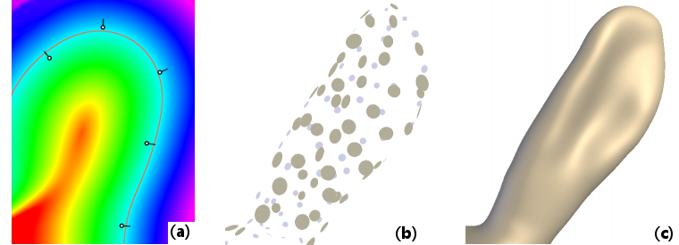
The fitting module is dedicated to the smooth fitting of point clouds and extraction of useful geometric properties. Figure 1(a) shows a typical example in 2D: we reconstruct a potential function (shown in fake colors) from a few 2D points equipped with normals; then the 0-isoline of this potential gives us an implicit curve (in orange) from which we can readily extract further properties like curvature. A great benefit of this implicit technique [8] is that it works in arbitrary dimensions: Figures 1(b-c) show how we reconstruct an implicit 3D surface with the same approach, starting from a 3D point cloud. Working with meshes then simply consists of only considering their vertices.

Figure 1: (a) An implicit 2D curve fit to a 2D point cloud. (b) A 3D point cloud shown with splats. (c) An implicit 3D surface reconstructed from (b).

This is just the tip of the iceberg though, as we also provide methods for dealing with points equipped with non-oriented normals [5], techniques to analyze points clouds in scale-space to discover salient structures [13], methods to compute multi-scale principal curvatures [14] and methods to compute surface variation using a plane instead of a sphere for the fitting [15].

In the following, we focus on a basic use of the module, and detail how to:

create and use a fitting method
obtain the derivatives of fitting result
extend every part of the computationnal pipeline
run the code on a CUDA environment

As a prerequisite, please read Defining Points in Ponca in order to define the points on which the computation will be performed. For an exhaustive list of available methods, pleas read: Fitting Module: Reference Manual.

First Steps

Include directives

The Fitting module defines operators that rely on no data structure and work both with CUDA and C++. These core operators implement atomic scientific contributions that are agnostic of the host application. If you want to use the Fitting module, just include its header:

#include "Ponca/Fitting"

Definition of the Fitting object

The Fitting Object is what Two template classes must be specialized to configure computations.

The first step consists in specifying a weighting function: it defines how neighbor samples will contribute to the fit, as illustrated in Figure 2(a) in 2D. In this example, we choose a weight based on the Euclidean distance using Ponca::DistWeightFunc, remapped through a bisquare kernel defined in Ponca::SmoothWeightKernel:
using NeighborFilter = DistWeightFunc<Point, SmoothWeightKernel<Scalar>>;
The second step identifies a complete fitting procedure through the specialization of a Ponca::Basket. In our example, we want to apply an Ponca::OrientedSphereFit to input data points, which outputs an Ponca::AlgebraicSphere by default. This leads to the following specialization:
using Sphere = Basket<Point, NeighborFilter, OrientedSphereFit>;

See also: Fitting techniques Overview; Available Weighting kernel

Fitting Process

At this point, most of the hard job has already been performed. All we have to do now is to provide an instance of the weight function, where \(t\) refers to the neighborhood size, and initiate the fit at an arbitrary position \(\mathbf{p}\). In this example we traverse a simple array, and samples outside of the neighborhood are automatically ignored by the weighting function. Once all neighbors have been incorporated, the fit is performed and results stored in the specialized Basket object.

        Fit fit1;
        fit1.setNeighborFilter({fitInitPos, analysisScale});
        fit1.compute(vectorPoints);

Check fitting status

After calling finalize or compute, it is recommended to test the return state of the Fit object before using it:

FIT_RESULT eResult = fit.compute(vecs.begin(), vecs.end()); // or eResult = fit.finalize();
if(eResult == STABLE)                                       // or fit.isStable()
      //do your things...

Warning: You should avoid data of very low (i.e., 1 should be a significant value) or very high (e.g., georeferenced coordinates) magnitude to get good results; thus global rescaling might be necessary.

Basic Outputs

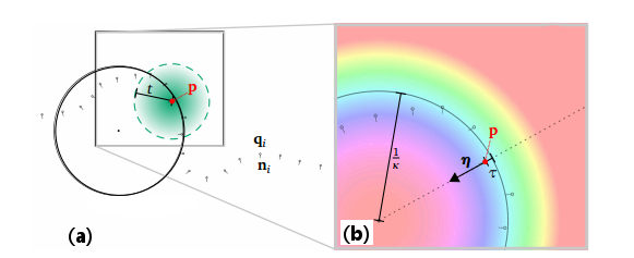
Figure 2. (a) Fitting a 2D point cloud of positions and normals at a point p (in red) requires to define a weight function of size t (in green). (b) This results in an implicit scalar field (in fake colors), from which parameters of a local spherical surface can be extracted: an offset tau, a normal eta and a curvature kappa.

Now that you have performed fitting, you may use its outputs in a number of ways (see Figure 2(b) for an illustration in 2D).

You may directly access generic properties of the fitted Primitive:

cout << "Value of the scalar field at the initial point: " << p.transpose()
     << " is equal to " << fit.potential(p) << endl;
cout << "Its gradient is equal to: " << fit.primitiveGradient(p).transpose() << endl;

This generates the following output:

Value of the scalar field at the initial point: 0 0 0 is equal to -0.501162

Its gradient is equal to: 0.00016028 0.000178782 -0.000384989

You may rather access properties of the fitted sphere (the 0-isosurface of the fitted scalar field), as defined in AlgebraicSphere :

cout << "Center: [" << fit.center().transpose() << "] ;  radius: " << fit.radius() << endl;
cout << "The initial point " << p.transpose()              << endl
     << "Is projected at   " << fit.project(p).transpose() << endl;

You will obtain:

Center: [-0.000160652 -0.000179197  0.000385884] ;  radius: 1.00232
The initial point 0 0 0
Is projected at    0.353911  0.394765 -0.850088

See also: Capabilities of Fitting tools for information about outputs of Fitting objects.

Evaluation schemes and projection

Some ComputeObject provide projection operators, which allows to define Moving Least Squares (MLS) surfaces (see [12] and [6]). MLS surfaces are not defined explicitly, but rather implicitly by projection operators. Under the hood, projecting on a MLS surface require to iterate between successive local fits (handled by the ComputeObject) and projection step (handled by a projection operator, as detailed below). Ponca provide MLSEvaluationScheme to perform this evaluation. To evaluate a MLS surface, you only need a ComputeObject and a set of points:

mls.compute(fitMLS, vectorPoints);

The method MLSEvaluationScheme::compute can be customized by changing the projection operator (DirectProjectionOperator and GradientDescentProjectionOperator are currently available). The class also provide control over the iteration stopping criteria (convergence and maximum number of iteration).

For convenience, Ponca also provide SingleEvaluationScheme, which has the same API than MLSEvaluationScheme, but simply does a single fit without projection. It is literally defined as

        template <typename ComputeObject, typename IteratorBegin, typename IteratorEnd>
        PONCA_MULTIARCH inline FIT_RESULT compute(ComputeObject& co, const IteratorBegin& begin,
                                                  const IteratorEnd& end) const
        {
            return co.compute(begin, end);
        };

Computing derivatives

Ponca provides BasketDiff, a class to extend an existing Basket with differentiation tools. Given a specialized type TestPlane that performs covariance plane fitting (using Ponca::CovariancePlaneFit), and defined as follows:

using TestPlane = Basket<Point, NeighborFilter, CovariancePlaneFit>;

BasketDiff allows to extend this type to compute its derivatives in space and/or scale:

    using PlaneScaleDiff      = BasketDiff<TestPlane, FitScaleDer, CovariancePlaneDer>;
    using PlaneSpaceDiff      = BasketDiff<TestPlane, FitSpaceDer, CovariancePlaneDer>;
    using PlaneScaleSpaceDiff = BasketDiff<TestPlane, FitScaleSpaceDer, CovariancePlaneDer>;

Changing fitting process

Internally, Ponca::Basket process the neighbors sequentially, and the compute function is overall equivalent to

        Fit fit;
        fit.setNeighborFilter({fitInitPos, analysisScale});
        fit.init();
        for (auto it = vectorPoints.begin(); it != vectorPoints.end(); ++it)
            fit.addNeighbor(*it);
        fit.finalize();

More complex computational scheme are included within Ponca (e.g BasketComputeObject::computeMLS for Moving Least Square). Still this simplicity can be used to change how this function behave and tailor it to your needs.

Note: Some methods require multiple fitting passes, e.g. MongePatch. This is directly handled by the compute method. If you don't use it, you need to check if eResults == NEED_ANOTHER_PASS and repeat the addNeighbor()/finalize() steps. Don't forget to call startNewPass() at each iteration.

This also allows to use custom data structures in order to speedup computation. You may, for example exclude points you know won't be within the prescribed radius. For this reason, Ponca provide spatial structures that can be used to accelerate spatial queries. Consider for instance using the KdTree class with range queries:

        Fit fit3;
        fit3.setNeighborFilter({vectorPoints[i].pos(), analysisScale});
        auto neighborhoodRange = tree.rangeNeighbors(vectorPoints[i].pos(), analysisScale);
        fit3.computeWithIds(neighborhoodRange, vectorPoints);

Note: Currently, users need to ensure consistency between the query and the fit location/scale. This is expected to be fixed in the upcoming releases.

See also: Spatial Partitioning module

Defining a new neighbor filter

Neighbor filters are critical components of the library. Their main goal is to provide computation information on how much a point is considered to be a neighbor. This information is given through weights defined by the Filter and the Kernel. In additions, some filters may transform the neighbors, for instance to express relatively to the evaluation point. Perhaps the most common filter is DistWeightFunc, which filters out points that are too far and weight the other according to their distance from the evaluation position, and also translate neighbors in the local frame. Another alternative are the classes NoWeightFunc and NoWeightFuncGlobal, which do not filter any neighbor and offer control over the transformation of the neighbors.

See also: Available filters

Defining a new distance kernel

DistWeightFunc is defined from the euclidean distance field centered at the evaluation position (see DistWeightFunc::init()). Given a distance to this evaluation position, the weight is computed (see DistWeightFunc::w()) by applying a 1d weighting function defined as follows:

DistWeightFunc also provides computation of the first and second order derivatives of the weight, both in scale (DistWeightFunc::scaledw(), DistWeightFunc::scaled2w()) and space (DistWeightFunc::spacedw(), DistWeightFunc::spaced2w()), and their cross derivatives (DistWeightFunc::scaleSpaced2w()). Theses methods check if the weight kernels provides the appropriate derivatives.

Filter API

It is also possible to define new filter that could take into account any other desired parameter. The general API is:

The filter should extend either CenteredNeighborhoodFrame or GlobalNeighborhoodFrame. They help to express points in local coordinates, often relative to the evaluation location. CenteredNeighborhoodFrame helps with translation invariant filters. Its conversion function is simply \(x - p\), where \(X\) is the query point and \(p\) the evaluation location.
GlobalNeighborhoodFrame does not affect coordinates and points remains in the global domain.

Defining a new Estimator

The goal of the Fitting module is to provide lightweight, fast and generic algorithms for 3d point cloud processing. We mostly focus on local regression techniques, which are core components of surface reconstruction techniques [3] [8], geometric descriptors [13] [11] or shape analysis techniques [10]. Most of these techniques share similar computation, and can be combined in several ways. For instance, NormalDerivativeWeingartenEstimator estimates curvature values by analyzing the spatial derivatives of a normal field, and can be combined with any normal estimation technique providing spatial derivatives.

In order to ease the association of multiple computational components, the library is based on the Curiously Recurring Template Pattern (CRTP). In contrast with polymorphism, this method allows to combine multiple short computations without adding runtime overhead (both in terms of memory footprint and execution time). Instead, the combination of the computational components is performed and optimized when compiling the program, and thus require more memory and time for this stage.

Because of some properties of the C++ language, our classes does not inherit from a Base interface defining the API, but rather follows concepts, as described in fitting_concepts.

Note: Beforing defining a new estimator, please take a look at Fitting techniques Overview and Capabilities of Fitting tools to learn more about available computation, their requirement and how to access their results.

Understanding CRTP in Ponca

The Basket class is the central part of the fitting module as it is the interface for all computation and provide the some utilities. The signature of the class is as follow:

template <class P, class NF, 
          template <class, class, typename> class Ext0,
          template <class, class, typename>... Exts>
class Basket;

The first two parameters are the Point type and the Filter used throughout the computation. The last two parameters defines the list of computation for each point cloud. Through multiple type indirection and type list unrolling, Basket will inherit all those Extension type in reverse order.

Unrolling example Ponca basic CPU, the basket is defined as:

using Fit1 = Basket<MyPoint, WeightFunc, OrientedSphereFit, GLSParam>;

This line, defines the class hierarchy:

Note: Some type are aggregates that will inject their dependancies within the class hierarchy. For example, OrientedSphereFit depends on MeanPosition, MeanNormal and AlgebraicSphere that appears in the class list although they were not explicitly defined by the user.

Because Basket inherit every types given as argument, it is easy to access any result or any set any parameter. It suffices to call the function on the Basket object as-if it was an object of the computation you want to alter.

The link between all these class is made through the defined Base type, which points to its parent class in the hierarchy. It becomes possible to access all result, all functions defined in the hierarchy through this prefix, provided there is no overriden name. Hence, in this example, refering to Base::m_uc within GLSParam will reference the current value of AlgebraicSphere::m_uc. However, refering to Base::addLocalNeighbor in GLSParam will reference the function OrientedSphereFitImpl::addLocalNeighbor as this is overriden by the class.

In order to target more directly a Fitting method, Ponca provides cast operation. For example, the MeanNormal class provide the MeanNormal::meanNormal function that returns a pointer to the implicit instance.

/* const */ MeanNormal* meanNormal = fit.meanNormal();

// Do whatever you want with a 'MeanNormal' instance

MeanNormal

Compute the mean normal of the input points.

Definition mean.h:85

Estimator API

Minimal requirements

In order to make an estimator compatible with Ponca Fitting API, new estimator should have the following structure:

        template <class DataPoint, class _NFilter, typename T = void>
        class ComputationalObjectConcept
        {
            // Defines common types (Base, Scalar, VectorType, NeighborFilter)
            PONCA_FITTING_DECLARE_DEFAULT_TYPES
        protected:
            enum
            {
                Check = PROVIDES_CAPABILITY_1 && PROVIDES_CAPABILITY_2    //< List of required capabilities
                                                     PROVIDES_CAPABILITY, //< List of provided capabilities
            };
 
        public:
            using Scalar         = typename DataPoint::Scalar;     //< Inherited scalar type
            using VectorType     = typename DataPoint::VectorType; //< Inherited vector type
            using NeighborFilter = _NFilter;                       //< Filter applied on the neighbors
        public:
            /**************************************************************************/
            /* Initialization                                                         */
            /**************************************************************************/
            // Init the WeightFunc, without changing the other internal states.
            // \warning Must be called be for any computation
            PONCA_MULTIARCH inline void setNeighborFilter(const NeighborFilter& _w);
 
            // Reset the internal states.
            // \warning Must be called before any computation
            PONCA_MULTIARCH inline void init();
 
            /**************************************************************************/
            /* Computations                                                           */
            /**************************************************************************/
            // Add a neighbor to perform the fit
            // \param w The weight of the point
            // \param lQ Local coordinates of the point (e.g.: the difference between the point and the eval position)
            // \param pt The point as defined by the user
            // \return false if param nei is not a valid neighbour (weight = 0)
            PONCA_MULTIARCH inline bool addLocalNeighbor(Scalar w, const VectorType& lQ, const DataPoint& pt);
            // \return State of fitting
            // \warning Must be called be for any use of the fitting output
            PONCA_MULTIARCH inline FIT_RESULT finalize();
        }; // class ComputationalObjectConcept

Note: The macro PONCA_FITTING_DECLARE_DEFAULT_TYPES defines the Base type (alias for T) as well as Scalar, VectorType and NeighborFilter for manipulation of related data. This macro is defined within <Fitting/defines.h>; If the estimator is expected to be the upmost parent of the hierarchy, do not inherit from T and default it to be void.

Warning: The macro PONCA_FITTING_DECLARE_DEFAULT_TYPES opens a public section.

In order for each computation to work properly, the functions init, addLocalNeighbor and finalize should call their Base version (Base::init, Base::addLocalNeighbor, Base::finalize). Presumably, this is among the first thing each of these function does.

Computational objets capabilities and requirements

Aggregating small computational objects allows to minimize code duplication, but also to easily combine different techniques. For instance, GLSDer can be used independently of the fitting technique, e.g. Ponca::OrientedSphereFit or Ponca::UnorientedSphereFit, as long as the fitted Primitive is an AlgebraicSphere.

In order to detect if the computational objects are correctly combined, Ponca provides a compile-time requirement/capability system: each computational objects check if the other classes of the CRTP provides the required computations. For instance, in the GLSParam class, we define the following enum:

    protected:
        enum
        {
            Check = Base::PROVIDES_ALGEBRAIC_SPHERE,
            PROVIDES_GLS_PARAMETRIZATION
        };

Base is a type defined from the CRTP and that represents the inherited classes. If Base does not define PROVIDES_ALGEBRAIC_SPHERE, this line generates an error when compiling the program. For instance, compiling the type

typedef Basket<Point, WeightSmoothFunc, GLSParam> FitSmoothOriented;

generates the following error:

Building CXX object /xxxxx/wrongType.cpp.o
In file included from /xxxxx/wrongType.cpp:19:
/xxxxx/ponca/Ponca/src/Fitting/gls.h:51:23: error: no member named 'PROVIDES_ALGEBRAIC_SPHERE' in 'Ponca::PrimitiveBase<PointPositionNormal<float, 3>, Ponca::DistWeightFunc<PointPositionNormal<float, 3>, Ponca::SmoothWeightKernel<float> >, void>'
        Check = Base::PROVIDES_ALGEBRAIC_SPHERE,
                ~~~~~~^

The capability PROVIDES_GLS_PARAMETRIZATION tells that GLSParam provides the GLS parameterization [13], and other components can access the related information.

In order to ease tools combinations, each class declare a set of required and provided capabilities, which are detailed in the Section concepts_provides.

Note: In its current version, the requirement/capability system offer limited protection over the combination of tools providing the same capabilities. Indeed, it is possible to build ill-formed combinations where two computations attempt to save their results at the same place, e.g. when using two fitting technique for the same primitive:
using Hybrid1 = Basket<Point, NoWeightFuncGlobal, Plane, MeanNormal, MeanPosition, MeanPlaneFitImpl,

CovarianceFitBase, CovariancePlaneFitImpl>; // test conflict detection in one direction

This case is not detected at compile time, but rather dynamically when calling finalize(), which returns CONFLICT_ERROR_FOUND. Internally, this is implemented by checking if the primitive is already valid (ie. it has been computed already) when finalizing the computation. This limitation is expected to be resolved in upcoming releases.

Providing cast operations

As explained earlier, the class hierarchy can not reach every function of every through the provided Base type due to overloading. The mecanism Ponca implements is a cast operator. Fortunately, this is quite common and a macro helps to define them. Add the following within a public section of your class:

  PONCA_EXPLICIT_CAST_OPERATORS(ClassName, className);
\encode
 
Where the first parameter is the class name and the second is the name of the cast function which is, most of the time, the same as the 
class name excpet a first lower case letter. Note that this macro requires the template parameter to be named following ponca conventions. 
 
\subsubsection fitting_newdiff New primitive differentiation (BasketDiff API)
  
The API for defining new estimator that differentiate the primitive follows the same principle from classical estimator. The base class is BasketDiff which follows the 
same CRTP / inheritance principle except that a Basket is required as a first parameter. 
 
\snippet concepts.hpp ComputationalDerivativesConcept
 
\note PrimitiveDer is the default entry point to most classes used in BasketDiff
 
A few addition should be notted however. First, the class is now templated on a flag (an integer) representing the variables according to which we want to differentiate. For now, 
Ponca defines only two set of variables (&lt;Fitting/enums.h&gt;):
 
- FitScaleDer: The derivatives of the primitive parameters w.r.t the scale (the neig radius)
- FitSpaceDer: The derivatives of the primitive parameters w.r.t the position of evaluation
- FitScaleSpaceDer: Compute derivative for both types. 
 
The macro `PONCA_FITTING_DECLARE_DEFAULT_DER_TYPES` defines two additionnal types `ScalarArray` and  `VectorArray`. Those types defines storage for derivative result. Note that 
they are fixed-size array whose size is adapted to the total number of derivatives. Their layout is described below depending on the type of differentiation. 
 
<table>
    <tr>
        <th>Fitting derivative value</th>
        <th>Number of derivatives</th>
        <th> Scalar Array indices </th>
    </tr>
    <tr>
        <td>FitScaleDer</td>
        <td> 1 </td>
        <td> [0] is the derivative w.r.t scale </td>
    </tr>
    <tr>
        <td> FitSpaceDer </td>
        <td> DataPoint::Dim </td>
        <td> [0:DataPoint::Dim] derivatives w.r.t eval position </td>
    </tr>
    <tr>
        <td> FitScaleSpaceDer </td>
        <td> 1 + DataPoint::Dim </td>
        <td> [0] derivatives w.r.t scale, <br/> [1:DataPoint::Dim+1) derivatives w.r.t eval position </td>
    </tr>
</table>
 
 
\section fitting_advanced Advanced usage
 
\subsection fitting_multiprimitive Fitting with multiple primitives
In most cases, only one primitive is included in the Basket, and it is recommended to use the helper classes provided by Ponca for fitting, e.g. CovariancePlaneFitImpl, OrientedSphereFitImpl.
However, Ponca also allows to combine multiple primitives, for instance to share intermediate computation results.
Using this functionality requires to really understand how the different primitives and fitting techniques are working.
In any case, it is recommended to explicitly define the computational arrangement, e.g.:
\snippet basket.cpp HybridType
 
After fitting, this object provides access to both the plane and the sphere, through the respective cast operators #AlgebraicSphere::algebraicSphere() and #Plane::plane().
 
\section fitting_cuda Cuda
Ponca can be used directly on GPU, thanks to several mechanisms:
 - Eigen Cuda capabilities, see <a href="http://eigen.tuxfamily.org/dox-devel/TopicCUDA.html"  target="_blank">Eigen documentation</a> for more details.
 You *need* to use a consistent `Eigen::Index` on both CPU and GPU if you plan to transfer memory between the computing units.
 That's why we recommend to set the following preprocessor variable when compiling your project:
 \code -DEIGEN_DEFAULT_DENSE_INDEX_TYPE=int

You might also need to define the --expt-relaxed-constexpr preprocessor option for NVCC. Example of working cmake file (see Screen Space Curvature using Cuda/C++):

enable_language(CUDA)
add_executable(ponca_ssgls "ponca_ssgls.cu")
target_compile_options(ponca_ssgls PRIVATE --expt-relaxed-constexpr)

Automatic CPU/GPU compilation qualifiers. We use the macro
PONCA_MULTIARCH void function();

to use the same code for C++ and CUDA. It has no effect when the code is compiled with GCC or Clang, but it will force the compilation for both host and device architectures when compiling with nvcc. A similar macro system is provided for mathematical functions, to switch between STL and CUDA versions.

Check the C++/Cuda and Python/Cuda (using PyCuda) examples for more details and how-to.

[Go to concept page] [Go back to user manual]

Table of Contents